Lab 2
Lab Goals
Test and familiarize yourself with the sensors and signal processing needed for your robot to detect acoustic and optical signals and interface with the Arduino Uno. The Acoustic sub-team will work on the microphone circuit, which will detect a 660 Hz whistle blow, signifying the start of the maze mapping competition. The Optical sub-team will work on the IR sensor circuit, which will detect nearby robots emitting IR at 6.08 kHz and distinguish them from decoys emitting at 18 kHz.
Prelab
- Review documentation for the analog-to-digital converter on the ATmega328 (Arduino microcontroller)
- Review documentation for Open Music Labs Arduino FFT Library
- Read about Fourier Transforms
- Read about Fast Fourier Transforms (FFT)
- Find a website to generate the 660 Hz tone for testing
- Design simple analog amplifying and filtering circuits
Sub-Teams
To begin, we split into two groups of two. Each group progressed through the lab individually, as described below.
- Acoustic Team = Kenneth and Tyler
- Optical Team = Brian and Eric
FFT Analysis
Both the Acoustic and Optical parts of this lab used Fast Fourier Transforms (FFT) to determine the frequency components of the sampled input signal from the sensors. For pure sinusoids, this is not so difficult, as one can simply read off the period in the time domain. However, for more complicated signals, it is not necessarily clear what frequencies are present, and certainly not clear if a given frequency is present. To make this process easier, a signal can be inspected in the frequency domain.
In the frequency domain, we can observe a signals “spectrum”. A spectrum is an interpretation of a signal which assigns a magnitude (an importance) to a given frequency. The standard way to compute this is with a Discrete Fourier Transform (DFT):
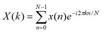
The DFT equation
The DFT computes a change of basis, assigning the weight X(k) to a given radial frequency (2*pi*k/N) by computing the inner product of the original signal with the complex exponential at that frequency.
Note that to compute one X(k) value, we need N multiplications, and N - 1 additions. To get useful information about a signal of size N, you generally need N values of k. This makes the DFT computation an O(n^2) operation, which can get very slow for large values of N.
To speed this process up, the Fast Fourier Transform (FFT) is used. The FFT is an algorithm for computing the DFT efficiently—the best speed up is achieved when N is a power of 2. The algorithm uses a “divide-and-conquer” method to compute the DFT. It first isolates the even and odd terms of the original DFT sum. Then it evaluates these sums as two independent FFTs of length N/2.
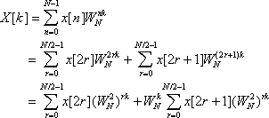
The FFT divide-and-conquer approach
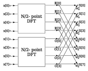
FFT Butterfly diagram
A key to this process is that the odd sum gets transformed into a N/2 FFT by pulling out an overall constant phase. This process of splitting up into two FFTs can continue down all the way until you have reached a series of FFTs, each acting on only two values. This splitting action occurs log2(N) - 1 times. At each stage, there are N multiplications and additions, so our computational complexity has decreased to O(N * log2(N)).
The FFT algorithm was implemented using Open Music Labs Arduino FFT
Library. By default, the library takes in an analog signal from Arduino
pin A0, samples it at 256 equally spaced intervals, and returns an array
with 128 values, which represent the magnitude of the frequency content
for frequenices up to half of the samping frequency. Since the FFT of a real signal is
symmetric over zero, only half of the outputs are unique, and thus 128
bins are returned (not 256).
The FFT code can be modified to alter the performance of the ADC
(information from the ADC section of the ATmega328 datasheet [page 305]).
The important ADC characteristics are:
- 10-bit resolution
- ADC clock is dependent on chosen prescalar, which is set based upon last 3 bits of ADCSRA register
- The default FFT code sets the ADC prescaler = 32
- Prescalar = 128 -> maps to clock of 125 kHz
- Prescalar = 64 -> maps to clock of 250 kHz
- Prescalar = 32 -> maps to clock of 1 MHz
- Prescalar = 16 -> maps to clock of 2 MHz
- Prescalar = 8 -> maps to clock of 4 MHz
- Prescalar = 4 -> maps to clock of 8 MHz
- NOTE - at frequencies higher than 250 kHz the 10-bit accuracy degrades
- A normal conversion takes 13 ADC clock cycles
- Sampling frequency = clock rate divided by number of cycles
- Fs = clock rate/cycles
- Fs = 125000/13 = 9615 Hz
Acoustic Team
GOAL: use an Arduino and the FFT library to detect a 660 Hz whistle blow
Materials Used
- 1 × Arduino Uno
- 1 × USB A/B cable
- 1 × Electret Condenser Microphone (CMA-4544PF-W)
- 1 × LM358 Op Amp
- 1 × 1 μF Polarized Capacitor
- 1 × 220 pF Capacitor
- 1 × 330 pF Capacitor
- 1 × 330 Ω resistor
- 1 × 3.3 kΩ resistor
- 1 × 3.9 kΩ resistor
- 2 × 10 kΩ resistors
- 1 × 390 kΩ resistor
- 2 × 680 kΩ resistor
- 1 Solderless breadboard
Testing the Microphone - Datasheet Circuit
- First, we built the recommended circuit from the datasheet to connect the microphone to the Arduino
- 1 × 1 μF Capacitor
- 1 × 3.3 kΩ resistor
- We used the previously mentioned website to generate a 660 Hz tone
- Results shown by the oscilloscope indicate a response, although the waveform amplitude is relatively small
- DC bias ~3mV
- Peak-to-peak ~40mV
- That is with the source right next to the microphone
- Clearly, we need to amplify the output
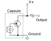
Circuit from datasheet

Circuit on breadboard
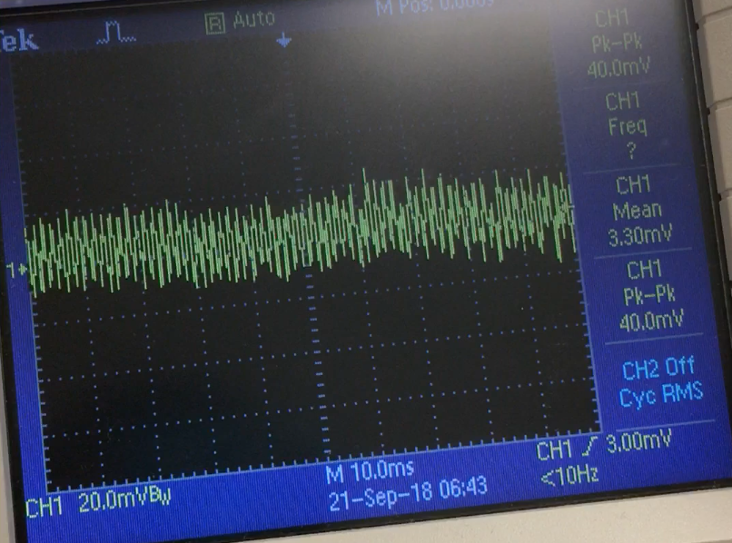
Results from oscilloscope
Testing the FFT Library
- As mentioned earlier, we use the Open Labs Arduino FFT Library for calculating the FFT
- To increase the accuracy of our readings, we altered the ADC prescaler value
- Original: prescaler = 32 -> maps to clock of 1 MHz
- Modified: prescaler = 128 -> maps to clock of 125 kHz
- The original code had:
- First set line: ADCSRA = 0xe5
- Second set line: ADCSRA = 0xf5
- Our modified code is:
        void setup() {
          Serial.begin(115200);                     // use the serial port
          TIMSK0 = 0;                               // turn off timer0 for lower jitter - delay() and millis() killed
          ADCSRA = 0xe7;                            // set the adc to free running mode, set prescaler=128 (default e5=32)
          ADMUX = 0x40;                             // use adc0
          DIDR0 = 0x01;                             // turn off the digital input for adc0
        }
        void loop() {
          while(1) {                                // reduces jitter
            cli();                                  // UDRE interrupt slows this way down on arduino1.0
            for (int i = 0 ; i < 512 ; i += 2) {    // save 256 samples
              while(!(ADCSRA & 0x10));              // wait for adc to be ready
              ADCSRA = 0xf7;                        // restart adc --> set prescaler=f7=128 (default f5=32)
- ADC clock = 125 kHz
- ADC sampling = 13 clock cycles per read
- ADC sampling = 125 kHz/13 = 9,615.38 Hz
- Number of Samples = 256
- Bin Size = 9,615.38/256 = 37.56 Hz/bin
- Bin for 660 Hz = 660/37.56 = 17.57 --> Bin 18
- Experimentally, we found that 660 Hz is right on the border between Bins 18 and 19
- Thus, in our integrated detection code we check for a large magnitude in BOTH of these bins
Building a Microphone Amplifier Circuit
- For our circuit, we added an active low pass filter with a gain of -10 dB
- First, we added two large (680 kΩ) resistors to bias the op amp's inverting input to mid-rail (2.5V)
- Next, we biased the op amp's non-inverting input to mid-rail using two 10 kΩ resistors, so that we only amplified the differential changes due to the microphone
- Lastly, we added a parallel RC tank which acts as a low pass filter with a cutoff frequency of around 742 Hz
- Because there was no 550 pF capacitor in lab, we added a parallel combination of a 220 pF and a 330 pF capacitor to give us the desired cutoff frequency
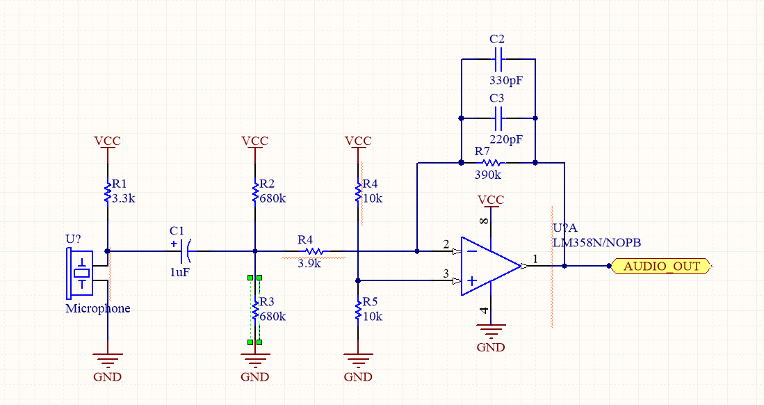
Circuit diagram
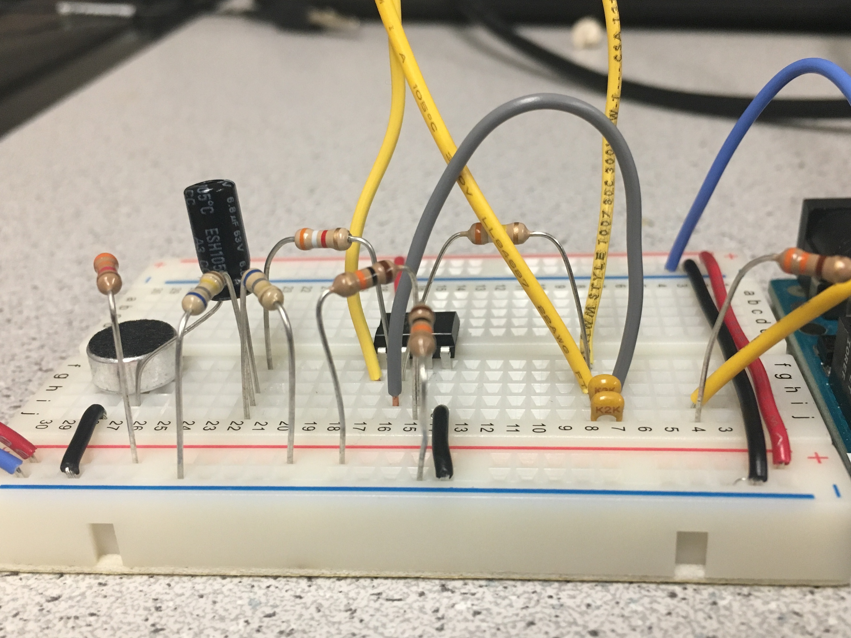
Breadboard circuit
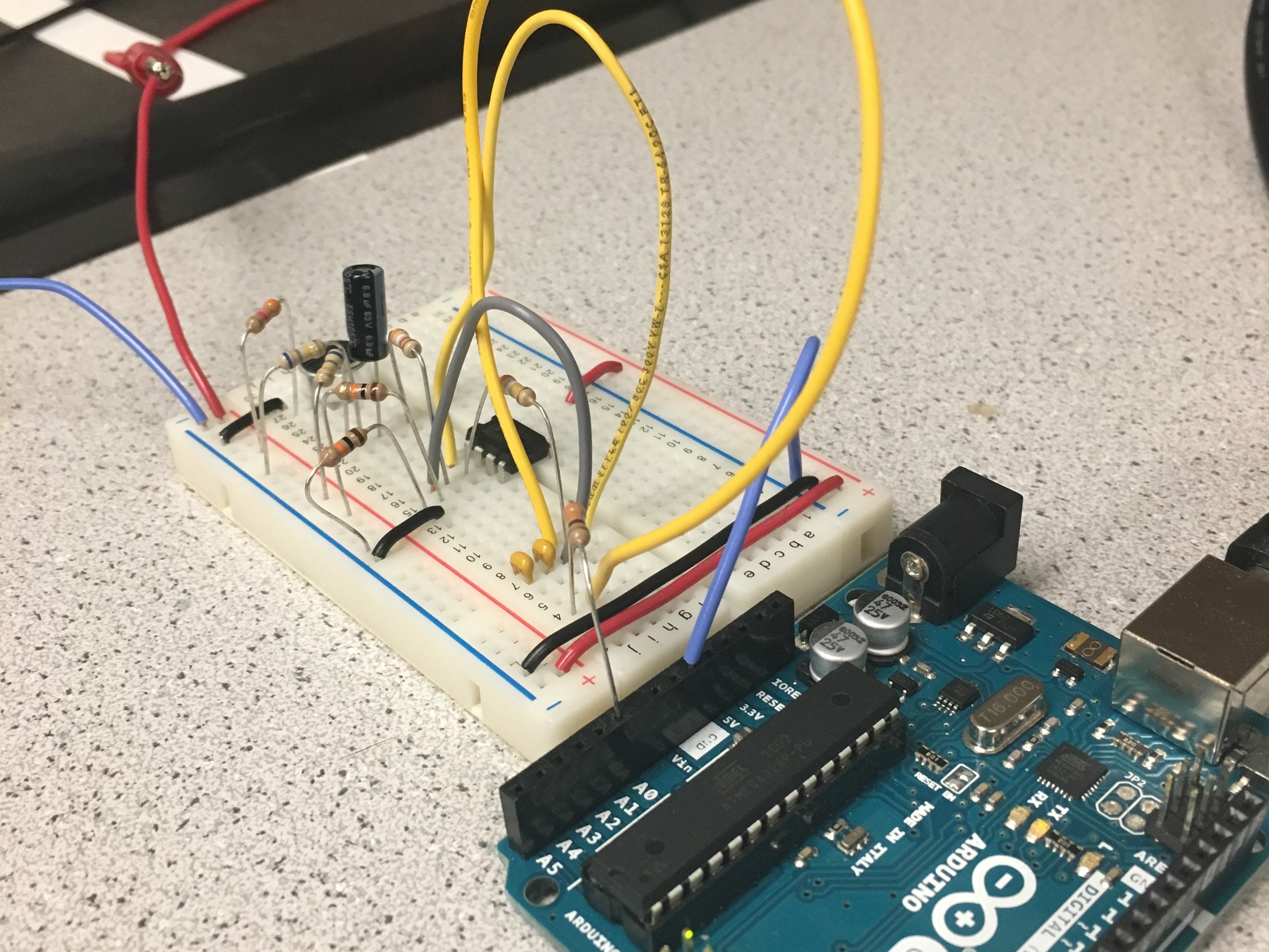
Breadboard circuit
Testing the Microphone - Amplifier Circuit
- Circuit testing
- To make sure the microphone amplifier circuit was working properly, we ran it through the following tests:
- 660 Hz tone
- 680 Hz tone
- 640 Hz tone
- 660+760 Hz tone
- 660+560 Hz tone
- For each test, we played one or more distinct tones from device(s) 5 cm away from the microphone
- With the audio playing, we ran the FFT code and recorded the data
- Once we finished, we graphed the results
- The data shows that we are successfully able to differentiate between various tones
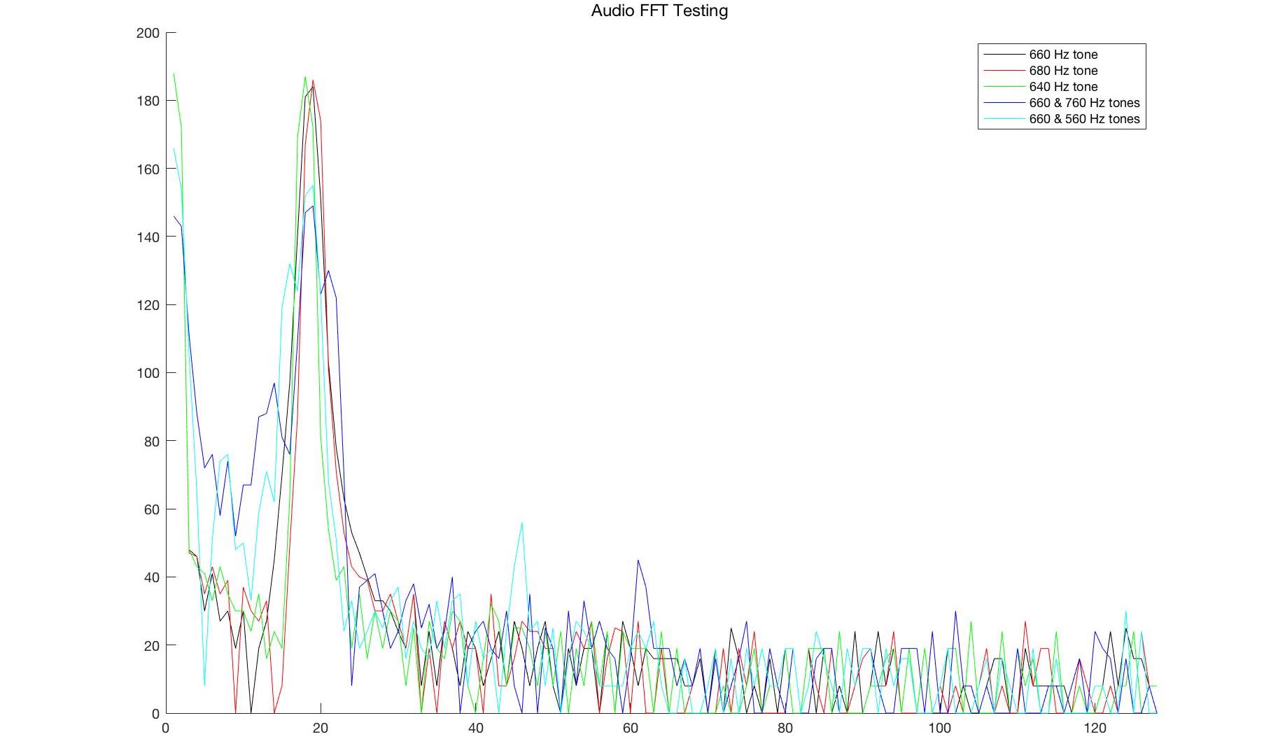
Microphone amplifier circuit FFT test results
Integrating the Microphone Functionality into Software
- We created a function "detect_660hz"
- Runs FFT function with prescaler = 128
- Checks bins 18 AND 19
- If magnitudes are both greater than a defined threshold -> returns TRUE
        /**
         * [detect_660hz]
         * OUTPUT = returns TRUE if a 660hz signal is detected by the Arduino,
         *          & FALSE otherwise
         * Uses THRESHOLD to determine whether the tone is playing or not
         */
        bool detect_660hz(){
            byte * fft_log_out = get_fft_bins();
            if (fft_log_out[17] > THRESHOLD && fft_log_out[18] > THRESHOLD) //bins 18 & 19, but 0 based so subtract 1
                return true;
            else
                return false;
        }
- Every time through the loop, "detect_660hz" is run
- To prevent a stray audio source from setting off our robot, a counter is used
- If and only if "detect_660hz" returns true 6 times in a row --> then the robot will start
- We showed this by turning the internal LED on
          #include "mic.h"
          #include "ir_hat.h"
          int counter = 0;

          void setup() {
            Serial.begin(9600);
            pinMode(LED_BUILTIN, OUTPUT);
            fft_setup();
          }
          void loop() {
            int count = 0;
            Serial.println(detect_660hz());
            if(detect_660hz())
              counter++;
            else
              counter = 0;
            if(counter>6)
              digitalWrite(LED_BUILTIN, HIGH);
            else
              digitalWrite(LED_BUILTIN, LOW);
          }
Demo:
Optical Team
GOAL: use an Arduino and the FFT library to detect another robot emitting IR at 6.08 kHz and ignore decoys (18 kHz)
Materials Used
- 1 × Arduino Uno
- 1 × USB A/B cable
- 1 × IR Phototransistor (OP598)
- 1 × IR hat (given by TAs)
- 1 × IR decoy
- 1 × LF353 Op Amp
- 1 × 2.3 μF Capacitor
- 1 × 10 nF Capacitor
- 1 × 10 Ω resistor
- 1 × 3.2 kΩ resistor
- 1 Solderless breadboard
IR Circuit Design
- We chose to implement an active band-pass filter with amplification in order to filter out DC and low frequency signals while also filtering out the higher frequency decoy signals
- Received IR signals in the pass band (from other robots’ IR hats) are amplified for better ADC quantization range, as well as to detect them from further distances
- Cut-off frequencies were intended to be 5 kHz and 7 kHz
- Our capacitor and resistor values were:
- R1 = 10 Ω
- C1 = 2.3 μF
- R2 = 3.2 kΩ
- C2 = 10 nF
- This resulted in cut-off frequencies of 4.97 kHz and 6.92 kHz
- The gain of the filter in the pass band was intended to be R2/R1 = 320
- Actual results:
- Peak Gain: 75 or 19 dB
- Bode Plot
- Shows bandpass filter with 3 dB bandwidth 700 Hz to 10 kHz
- 18kHz signal is half the power of the 6 kHz signal after active filter
- Harmonics of the 18 kHz signal that would alias into the 6 kHz bins come out of the filter with 1/10 the magnitude of a 6 kHz signal
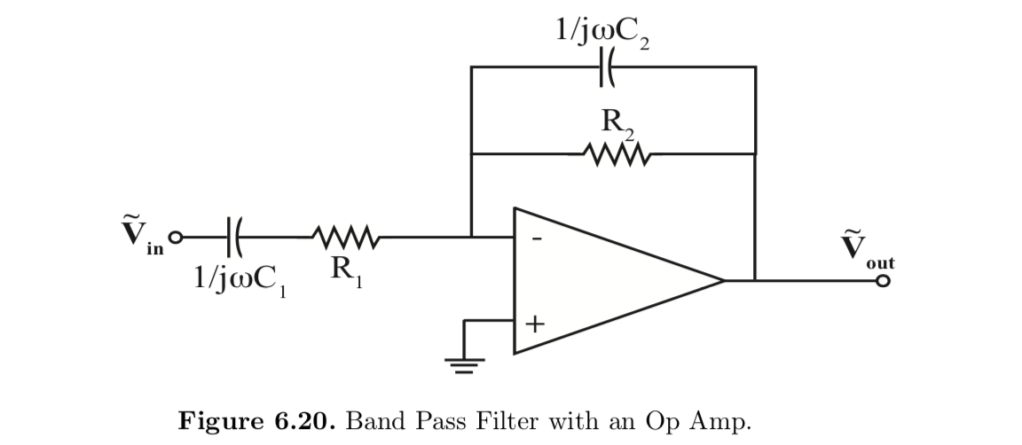
Band-pass filter schematic (from Professor Shealy, ECE2100 course notes)
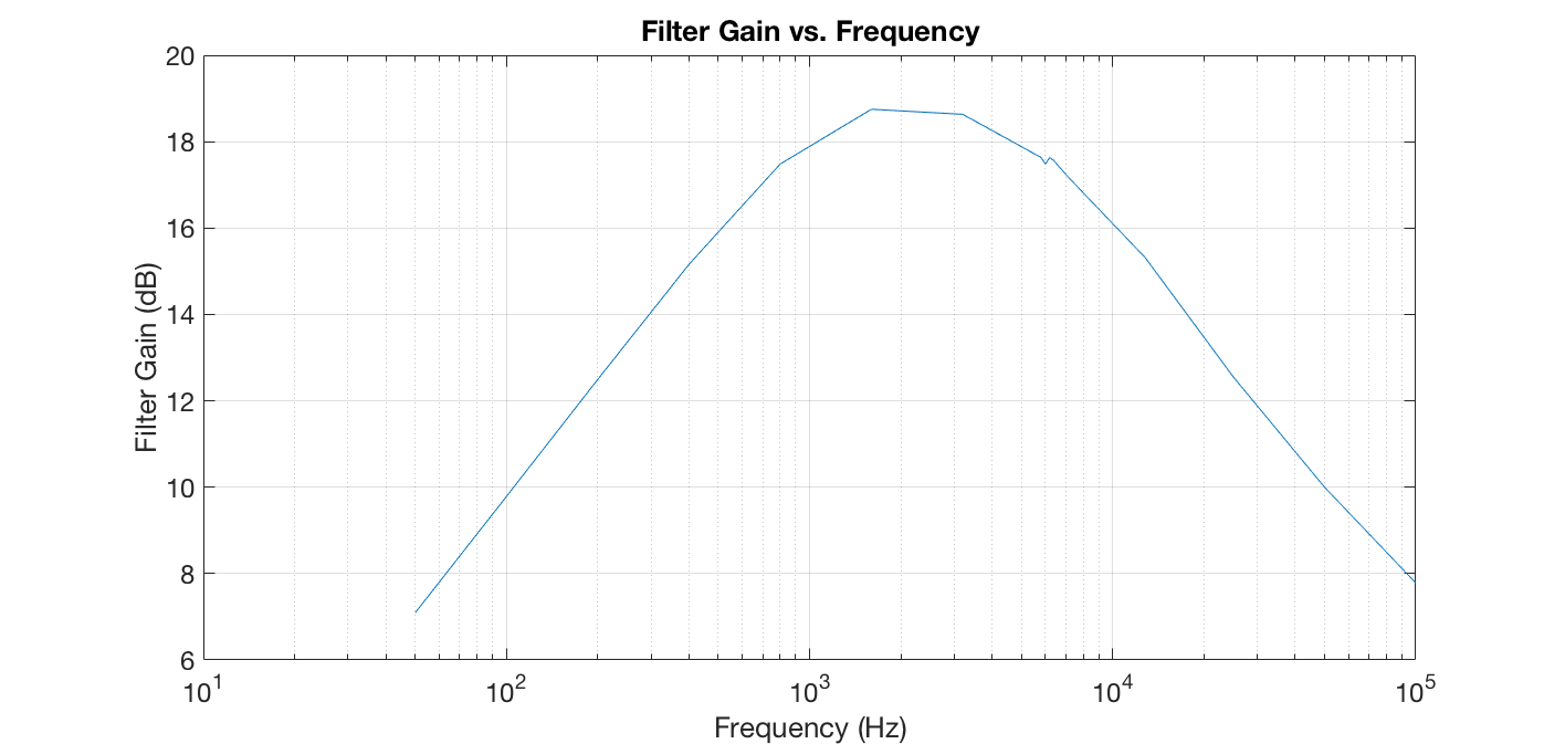
IR filter bode plot
FFT Analysis
- The default example code sets the ADC in free running mode and polls for each ADC conversion
- ADC prescaler = 32
- NOTE - this ADC setup is different from the one used by the Acoustic Team
- Arduino clock frequency = 16 MHz
- Thus, sampling frequency = 38.4 kHz
- This is quick enough for the purpose of detecting IR signals, since we are sampling above the Nyquist rate, and the highest frequency IR signal we will see is 18 kHz
- However, we may still see harmonics of these signals that are aliased to lower frequencies, since a sinusoidal input to a diode will cause harmonics
- Given our sampling rate and decoy frequency, we expect these aliased signals to appear at frequencies that are filtered out by our band pass filter
- The FFT code outputs 128 bins
- Frequencies of interest are in bins 41 and 42
- This corresponds to 6.01 kHz and 6.16 kHz
Results
Silence
- Spectrum is pretty sparse
- There are some small peaks around 8 kHz and 13 kHz
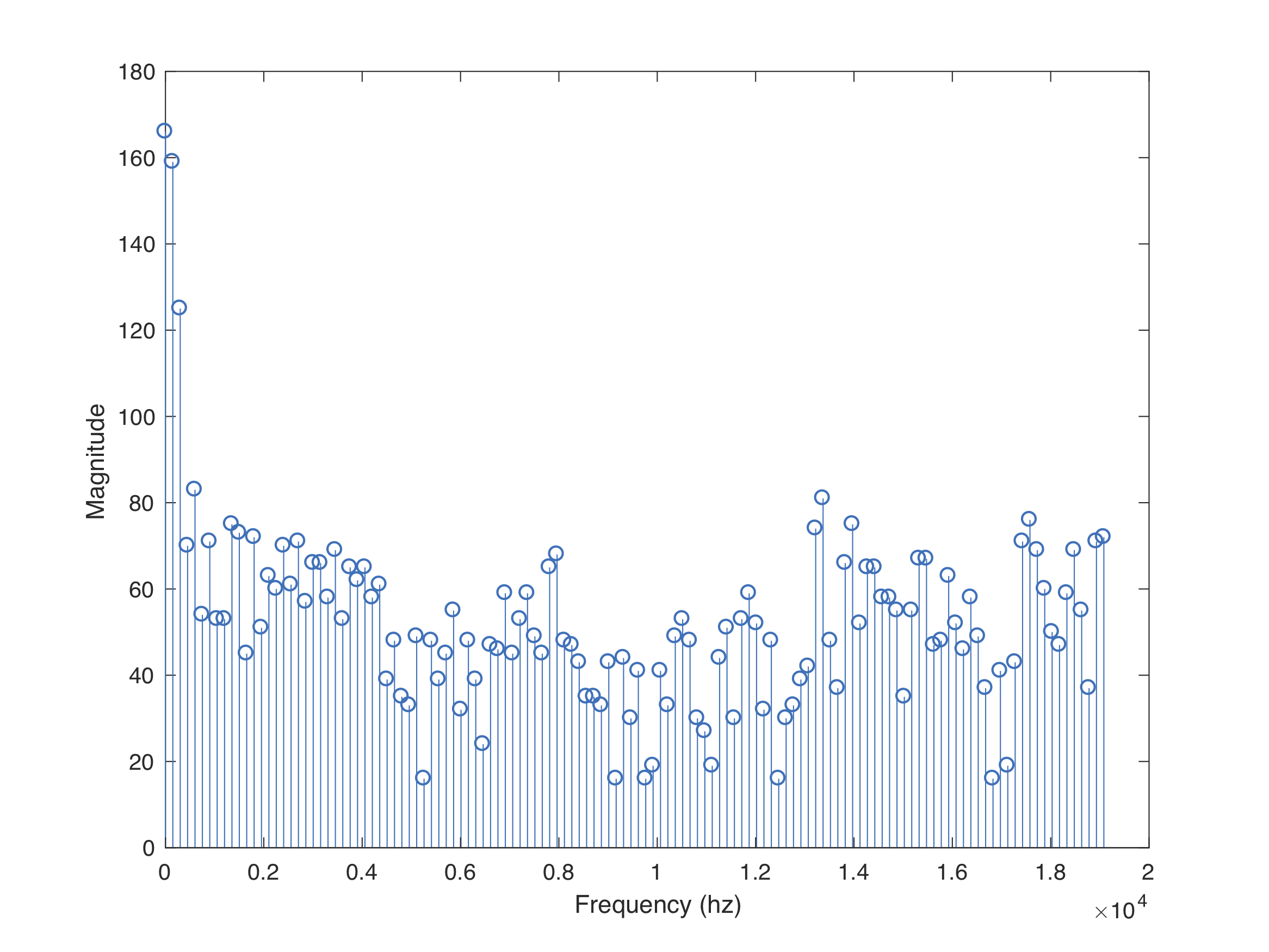
IR Hat
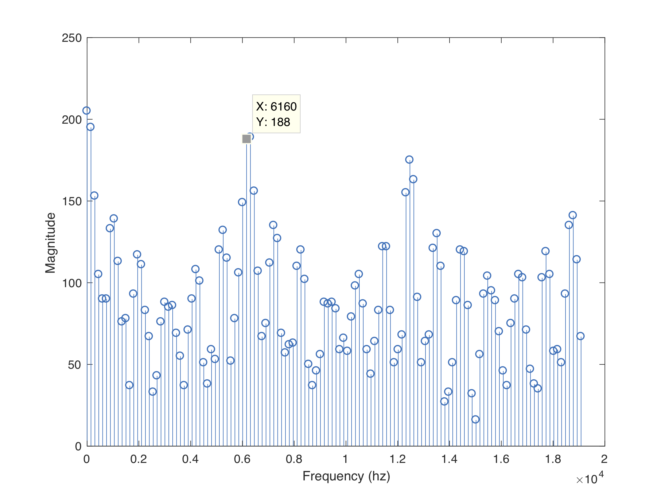
- There is a large peak at 6160 Hz
- Bins 41 and 42 correspond to the 6 kHz IR hat signal
- When the peaks in these bins are above a threshold, then the IR hat signal is detected
IR Decoy
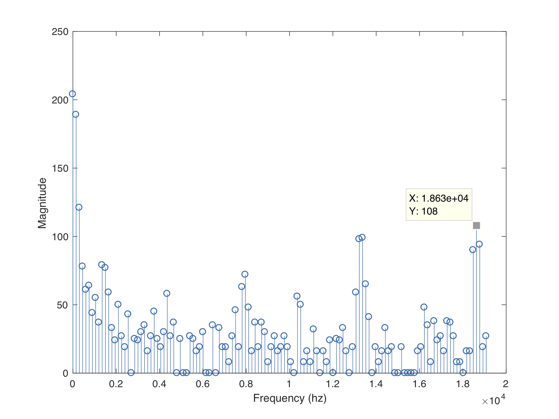
- There is a peak corresponding to 18 kHz on the spectrum
- No frequencies are aliased to the bins around 6 kHz
- Thus, we can ignore the 18 kHz peak and only observe bins 41 and 42 for IR hat detection
IR Hat + IR Decoy
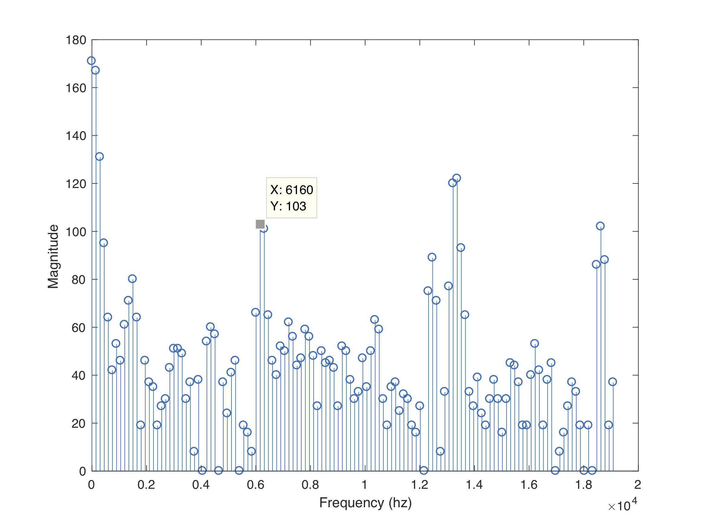
- There are peaks at 6 kHz and 18 kHz
- Ignore the 18 kHz bins
- Observe bins 41 and 42 for IR hat detection
Concurrent Testing
Our concurrent testing software works as follows
- Idle until 660 Hz tone is detected
- When microphone circuit detects 660 Hz, turn on YELLOW LED and advance in code
- Continuously run IR detection code
- If 6.08 kHz IR is detected, turn on GREEN LED